
Binaural source localization: estimate a source's azimuth from a room impulse response (BRIR).
files
readme.md
Localizer
Estimate where a sound source sits in space from a Binaural Room Impulse Response (BRIR).
Given a BRIR — the two-channel impulse response of a loudspeaker captured at a listener's two ears in a real or simulated room — Localizer estimates the azimuth of the source: its lateral angle (left ↔ right) and its front/back hemisphere. Elevation is not estimated.
The design philosophy is to model human binaural hearing rather than to invert the room acoustics. Localizer extracts the direct-sound Head-Related Impulse Response (HRIR) from the BRIR, computes the same binaural and monaural cues the auditory system uses to localize sound, and matches them against a reference database of measured HRTFs to find the most similar direction.
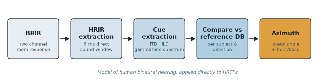
Background: how humans localize sound
The auditory system has no direct "direction sensor". Instead it infers direction from three physical cues produced as a sound wave interacts with the head, torso and outer ears:
| Cue | Physical origin | What it disambiguates |
|---|---|---|
| ITD — Interaural Time Difference | The far ear is a longer path from the source, so the wave arrives later (up to ~0.7 ms for a human head). | Left ↔ right (dominant below ~1.5 kHz). |
| ILD — Interaural Level Difference | The head acoustically "shadows" the far ear, more so at high frequencies where the wavelength is small relative to the head. | Left ↔ right (dominant above ~1.5 kHz). |
| Spectral cues (monaural) | The pinna, head and torso filter the incoming sound direction-dependently, imprinting peaks and notches on its spectrum. | Front ↔ back and elevation. |
This division of labour — binaural cues (ITD/ILD) for left/right, spectral cues for front/back — is Duplex Theory (Lord Rayleigh, 1907) extended with the monaural spectral mechanism. Localizer mirrors it directly.
The whole direction-dependent filtering is captured by the Head-Related Transfer Function (HRTF) — the frequency response from a source at a given direction to each eardrum — whose time-domain form is the HRIR. A BRIR is essentially an HRIR followed by the room's reflections and reverberation.
The front/back ambiguity
ITD and ILD alone cannot separate front from back. A source in the frontal hemisphere and its mirror image behind the interaural axis produce (to first order) the same ITD and ILD — they lie on the same "cone of confusion". The figure below shows this for a simplified head model: the source at 30° and its rear mirror at 150° sit on top of each other in both cues.
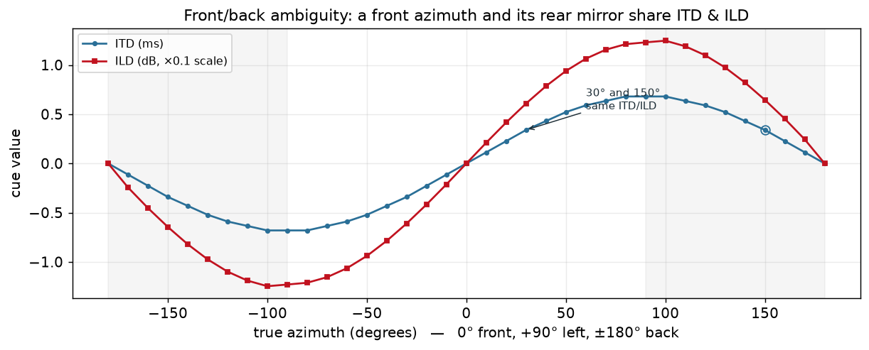
Resolving front from back therefore requires the monaural spectral cue — which is exactly what the specialized approach (and, optionally, the CNN) use.
Method
1 · HRIR extraction · localizer/extraction.py
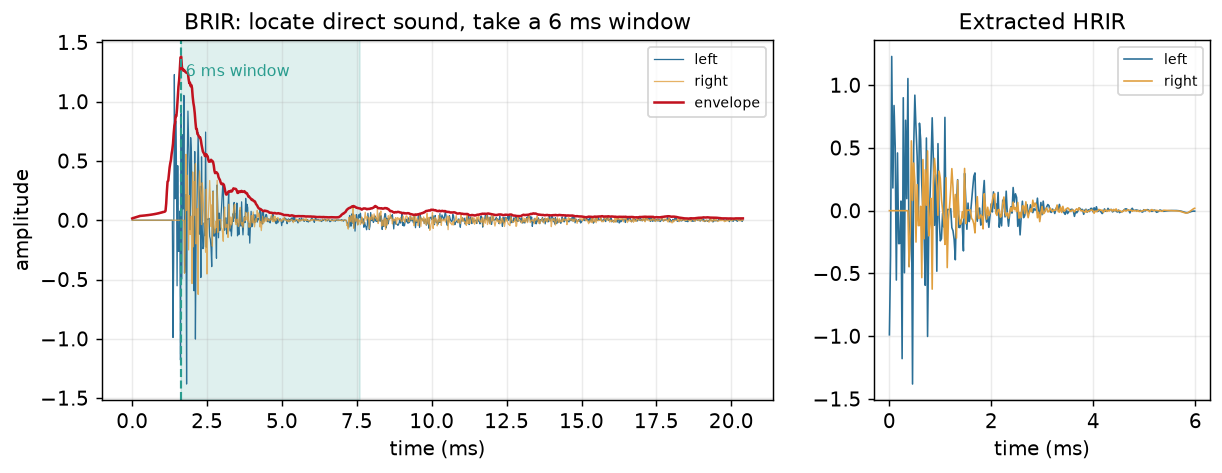
A BRIR is the direct sound (whose leading portion is, to a good approximation, the source's HRIR) followed by early reflections and a reverberant tail. Only the direct-sound HRIR carries clean directional cues, so we isolate it:
- Compute the amplitude envelope of the summed channels (via the analytic/Hilbert
signal) and find its first maximum — the arrival of the direct sound.
- For each channel, find the first envelope minimum after that maximum — the end of that
channel's direct HRIR. The two channels may end at different samples; that offset is the interaural delay itself.
- Low-pass filter the tail of the window, so slow low-frequency content is preserved
while treble bleed from the onset of the first reflection is attenuated. (High frequencies are expressed in fewer samples than low ones, and an HRTF's treble is where the sharpest direction-dependent features live.)
- Iteratively trim to a fixed length (6 ms, ≈256 samples at 44.1 kHz), each step
dropping whichever end contributes less energy — which also removes any leading silence.
Six milliseconds is a deliberate compromise: long enough to contain the direct sound and its HRIR, short enough to usually exclude the first reflection. (For scale, MIT-KEMAR ships 12 ms raw / 3 ms compact HRIRs.)
2 · Auditory filterbank · localizer/gammatone.py
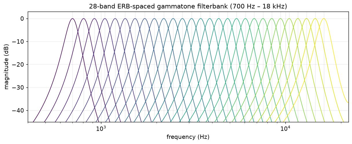
Each channel is decomposed into 28 frequency bands using a gammatone filterbank whose centre frequencies are spaced on the ERB (Equivalent Rectangular Bandwidth) scale from 700 Hz to 18 kHz. A gammatone filter approximates the frequency selectivity of a single place on the basilar membrane; an ERB-spaced bank therefore approximates the cochlea's roughly logarithmic frequency resolution.
The implementation is Slaney's fourth-order gammatone realised as a cascade of four second-order sections (Apple Tech. Report #35, 1993), self-contained with no third-party gammatone dependency. Each band is normalised to unit gain at its centre frequency:
3 · Cue extraction · localizer/cues.py
From the band decomposition and the two channels we compute:
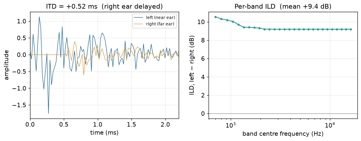
- ILD — the per-band RMS level difference (left − right) in dB → a 28-element vector.
- ITD — the global left/right delay, taken as the lag maximising the cross-correlation of
the two channels, converted to seconds. (Positive ITD ⇒ right ear delayed ⇒ source on the left.)
- Spectral representation — the per-channel band levels, normalised (zero-mean).
Normalising markedly improves front/back robustness and keeps measured-vs-reference comparison stable across different sample rates.
4 · Similarity & azimuth · localizer/similarity.py
Reference HRTFs are organised by subject; each subject contributes HRIRs at many directions. For the target HRIR and each reference (template) HRIR of a subject we form:
Δ_ITD       = | ITD_template − ITD_target |
Δ_ILD       = mean( | ILD_bands_template − ILD_bands_target | )
Δ_spectral  = mean( | spectrum_template − spectrum_target | )     (inter-spectral difference)
Δ_ITD and Δ_ILD are min–max normalised across each subject's directions so that subjects with different overall cue ranges are comparable, then combined into a similarity score. Two approaches are provided:
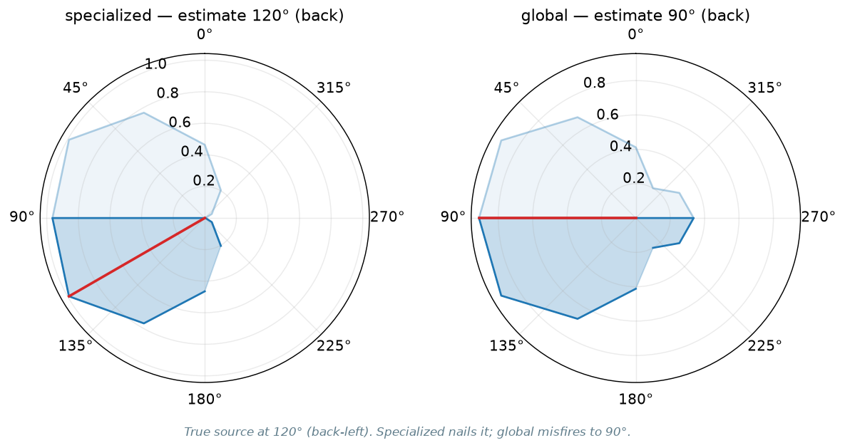
- Global — a single score over the full 360°:
sim = w_ITD·(1 − Δ_ITD) + w_ILD·(1 − Δ_ILD) + w_spec·(1 − Δ_spectral)
- Specialized (default, more accurate) — the lateral angle is estimated from
ITD + ILD only; the front/back hemisphere is decided separately from the spectral cue (specifically the standard deviation of the inter-spectral difference between the two ears). This matches how the auditory system treats binaural and monaural cues independently.
Per-subject similarity curves are aggregated across subjects either by averaging or by voting (each subject's winning angle scores a vote), and the winning azimuth is read off.
The polar plot below shows why the split helps. For a true source at 120° (back-left), the specialized approach localises it exactly, while the single 360° score of the global approach is pulled toward the front mirror and lands at 90°:
5 · CNN front/back · localizer/cnn.py (optional)
Because ITD and ILD cannot separate front from back, the front/back decision is the weakest link. A small 1-D convolutional network can learn it directly from the raw two-channel HRIR, using the monaural spectral information end-to-end:
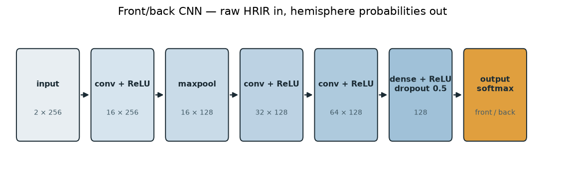
Input is the extracted HRIR as 2 channels × 256 samples; convolutional layers with ReLU activations (the first followed by max-pooling); 50 % dropout before the final dense layer; two outputs = P(front), P(back). The model definition and a training scaffold (localizer/cnn_train.py) are included. It ships untrained — the large multi-database HRTF corpus it needs is not distributed here — and the rest of the pipeline works without it.
Installation
python -m venv .venv && source .venv/bin/activate
pip install -e ".[sofa,gui,ml,dev]"    # extras: sofa, gui, ml (torch), dev (pytest)
The core install (pip install -e .) needs only numpy, scipy, soundfile and matplotlib. The extras are independent — install only what you need.
Usage
Command line
# One BRIR against a reference database, printed as a table
localizer analyze room_az030.wav --db path/to/hrtf_db

# A whole folder of BRIRs, as JSON, with a summary plot per file
localizer analyze brirs/ --db path/to/hrtf_db --json --plot-dir out/

# Using a trained front/back CNN
localizer analyze brirs/ --db path/to/hrtf_db --cnn-weights frontback.pt
Desktop GUI
localizer-gui # or: python -m localizer.guiLoad a database directory, then open a BRIR. The window shows the estimated azimuth and hemisphere for both approaches, the polar similarity plot, the extracted HRIR waveform, and the gammatone spectrum.
Python API
from localizer.pipeline import Localizer

loc = Localizer.from_database_path("path/to/hrtf_db")
result = loc.analyze_file("room_az030.wav")
print(result.specialized.azimuth, result.specialized.hemisphere)
print(result.summary())   # JSON-serialisable
Reference HRTF databases
Two formats are auto-detected by localizer/database.py:
- SOFA (AES69) — one
.sofafile per subject (needs thesofaextra). This is how most
public HRTF sets are distributed (e.g. IRCAM Listen, BiLi, CIPIC, ARI, RIEC). SourcePosition supplies azimuth/elevation and Data.IR the HRIRs.
- WAV folders — one sub-directory per subject holding WAV files named with their angle,
e.g. az030.wav or az-045_el00.wav (azimuth in degrees; +/- and an optional el elevation are accepted).
Only directions near the horizontal plane (elevation ≈ 0°) are used, since the model estimates azimuth.
Azimuth convention: 0° = front, +90° = left, ±180° = back, −90° = right (matching the polar plot, 0° at the top, counter-clockwise positive).
For validation, BRIR collections captured across many rooms/orientations (such as the ASH set, which aggregates BRIRs from several sources) provide known loudspeaker directions to compare against. These databases are large external downloads and are not bundled here.
Expected accuracy
On horizontal-plane BRIR sets with known loudspeaker directions, the specialized approach localises the lateral angle to within a few degrees on average and identifies the correct hemisphere for essentially all sources that are clearly front or back. Sources at exactly ±90° (directly to the side) and ±180° (directly behind, with zero ITD and ILD) are inherently ambiguous for front/back and are the expected failure points — the CNN is intended to help there. The global approach is consistently a little less accurate on both lateral angle and hemisphere, which is why the specialized split is the default.
The synthetic-fixture test suite (tests/) exercises the whole pipeline end-to-end — and all the figures above are generated from that same code via python docs/make_figures.py — so no multi-gigabyte HRTF download is needed to run or validate the project.
Corrections and design choices
- Distinct spectral weight. The global similarity formula uses its own weight
w_specon
the spectral term, not a reused ITD weight.
- Specialized approach as default. Estimating lateral angle and hemisphere separately is
both closer to human hearing and measurably more accurate than a single 360° score.
- Work directly on HRTFs, rather than on Directional Transfer Functions (after removing a
subject's Common Transfer Function). The DTF/CTF route is a known alternative from the elevation-localization literature; working on HRTFs keeps the pipeline self-contained.
- Normalised spectra for sample-rate robustness between measured and reference HRIRs.
Limitations
- Only the direct sound is analysed. Localizing early reflections is possible in principle by
applying the same method to each extracted reflection, but reliably isolating reflections from measured (as opposed to simulated) BRIRs is hard.
- A single source per BRIR is assumed. Perfectly synchronised sources fuse into one "phantom"
source (e.g. a centred image from a symmetric stereo pair) and are analysed as such.
- The model imitates human auditory localization, including some of its ambiguities; "true"
source direction and perceived direction need not coincide.
- The CNN needs a large, well-constructed training corpus to be effective; it ships untrained.
Development
pytest -q                              # run the test suite (37 tests)
python docs/make_figures.py            # regenerate the README figures
python -m localizer.cnn_train --db DB --out frontback.pt --epochs 20   # train the CNN
Repository layout
localizer/
  audio_io.py     WAV + SOFA loading, resampling
  extraction.py   BRIR → direct-sound HRIR (6 ms)
  gammatone.py    ERB-spaced gammatone filterbank
  cues.py         ITD, ILD, spectral representation
  database.py     reference HRTF database (SOFA / WAV folders)
  similarity.py   global + specialized scoring
  cnn.py          front/back CNN + inference wrapper
  cnn_train.py    CNN training scaffold
  pipeline.py     orchestration (BRIR → AnalysisResult)
  plotting.py     polar / waveform / spectrum plots
  cli.py          command-line interface
  gui.py          PySide6 desktop app
docs/make_figures.py   figure generation
tests/                 synthetic fixtures + 37 tests
References
- Lord Rayleigh (J. W. Strutt), "On our perception of sound direction," Phil. Mag. (1907) —
Duplex Theory of ITD/ILD.
- B. R. Glasberg & B. C. J. Moore, "Derivation of auditory filter shapes from notched-noise
data," Hearing Research (1990) — the ERB scale.
- M. Slaney, "An Efficient Implementation of the Patterson–Holdsworth Auditory Filter Bank,"
Apple Technical Report #35 (1993) — the gammatone filterbank.
- J. Blauert, Spatial Hearing (MIT Press, 1997) — HRTFs, cones of confusion, front/back.
- AES69 (SOFA) — Spatially Oriented Format for Acoustics, for HRTF/BRIR exchange.
License
MIT.